
Research note · Demand forecasting
Forecasting U.S. domestic flight volume with a seasonal ARIMAX model
Monthly arrivals are seasonal, capital planning is not. A model that carries the seasonal structure forecasts ten held-out months to within 1.72%; the same model without it misses by twice as much — and fails its residual diagnostics outright.
In brief
- Over January–October 2024, held out of estimation, the seasonal model's mean absolute percentage error was 1.72% — roughly 9,800 flights a month on a base near 580,000. The non-seasonal comparison model came in at 3.47%.
- The gap is not just accuracy. The non-seasonal model's residuals fail the Ljung–Box test (p ≈ 0), meaning structure is left unmodelled. It is misspecified, not merely less precise.
- Income matters more than fuel. GDP per capita enters the seasonal model significantly; the jet fuel spot price does not, once seasonality is accounted for. In the non-seasonal model the reverse appears — a sign the fuel term was absorbing seasonal variation.
- The pandemic is modelled, not deleted. A three-month dummy for March–May 2020 keeps the full series in the estimation window instead of discarding the shock.
01 Why forecast flight volume
Aviation runs on long-dated commitments. Fleet orders, lease terms, crew bases, and maintenance capacity are all decided years ahead of the traffic they serve, and each is expensive to reverse. The quality of those decisions depends on how well the operating envelope can be anticipated.
Commercial traffic is also a broad economic indicator in its own right, tracking both household income and business activity. Forecasting it well is therefore useful beyond the operations department — to lessors sizing residual values, to insurers pricing exposure, and to anyone underwriting a route.
The difficulty is that flight volume is shaped by forces outside the series: fuel costs, household income, and, once in a generation, a shock large enough to remove most of the traffic in a single quarter. This note asks a narrow question — can a standard time-series model, given a few economic inputs and an explicit allowance for the pandemic, forecast monthly U.S. domestic volume accurately enough to be worth using?
02 Data
The dependent series is the monthly count of completed domestic arrivals by U.S. carriers, published by the Bureau of Transportation Statistics, covering January 2010 to October 2024. Reporting carriers are those drawing at least 1% of passenger revenue from domestic scheduled service, plus voluntary filers.
Aggregating daily counts to monthly totals yields 178 observations. The first 168 (through December 2023) were used for estimation; the final ten (January–October 2024) were withheld entirely and used only to score the forecasts.
Exogenous inputs
Real GDP per capita proxies income and the willingness to travel. Jet fuel spot price proxies operating cost, which passes through to fares and, with a lag, to demand — an effect found to be asymmetric, with rises depressing demand more than falls stimulate it (Wadud, 2014).
A COVID peak dummy covers March, May and the month between — the WHO declared a pandemic on 11 March 2020, and those three months contain the steepest decline in the series. Isolating them lets the model absorb the shock without distorting the surrounding trend, and without discarding four years of subsequent data.
03 What the series shows
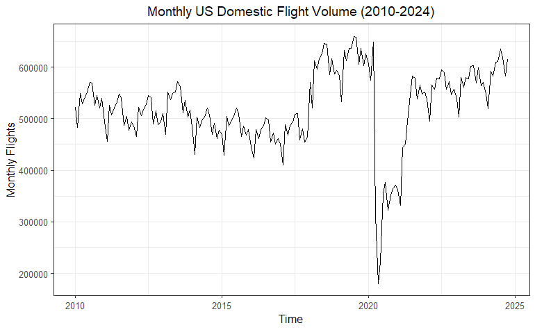
Three regimes are visible without any modelling. From 2010 to roughly 2017 volume oscillates in a band around 500,000 flights a month with no strong trend. From 2018 the level steps up. In March 2020 it collapses to under 200,000 — a decline the BTS put at 96% for April passenger traffic against the prior year — and then recovers over about eighteen months, reaching a level near the pre-pandemic peak by 2022 and holding there.
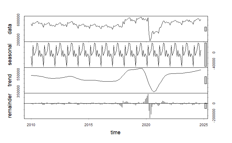
Decomposing the series separates what is routine from what is not. The seasonal component is strikingly regular: July and August peak, January and February trough, and the swing is worth roughly 50,000 flights a month, every year, including through the recovery. The trend component carries the 2020 collapse and the climb back.
The remainder is the informative panel. Before 2020 it is small and patternless, which is what a well-behaved series looks like. During 2020 it spikes hard — trend and season together cannot account for what happened, which is the empirical case for giving the pandemic its own term rather than hoping the model absorbs it.
04 Testing the series
Two stationarity tests were run on the levels series. The augmented Dickey–Fuller test returned p = 0.01, rejecting its null of a unit root. The KPSS test also returned p = 0.01 — but KPSS takes stationarity as its null, so that result rejects stationarity.
The models below were estimated on the levels series with no differencing (d = 0, D = 0), with the pandemic dummy carrying the shock. The disagreement between the two tests is noted rather than resolved.
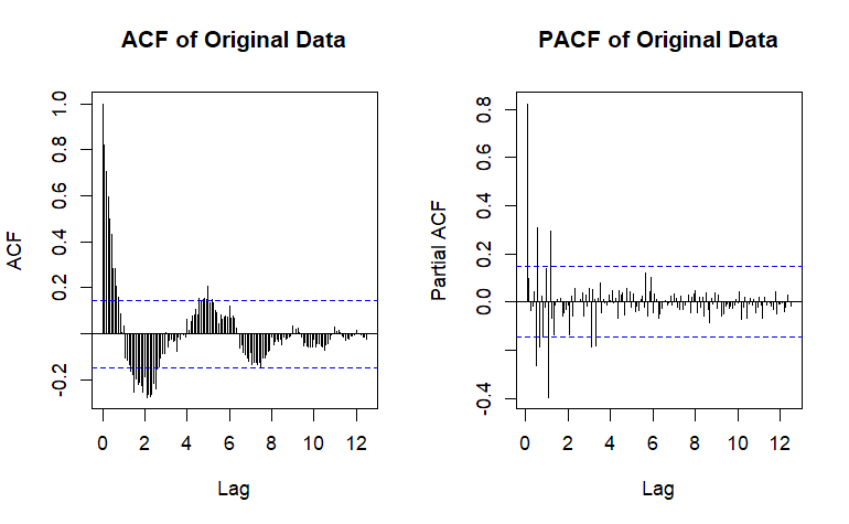
The correlograms suggest moving-average terms at the first two lags and an autoregressive structure decaying after lag 1. With exogenous regressors and seasonal structure both present, though, reading orders off these plots by eye is unreliable, so the orders were selected automatically instead.
05 Two models
Orders were chosen by auto.arima, which searches combinations of the non-seasonal (p, d, q) and seasonal (P, D, Q) parameters and keeps the lowest AIC. Two models were fitted: a seasonal specification, and — as a control — the same setup with the seasonal machinery removed.
Seasonal model — SARIMAX(1,0,2)(2,0,0)[12]
One autoregressive term, two moving-average terms, and two seasonal autoregressive terms at a twelve-month period, with no differencing on either side:
| Parameter | Estimate | Std. error | p | 5% |
|---|---|---|---|---|
| ar1 | 0.8877 | 0.0523 | 0.0000 | ● |
| ma1 | 0.4264 | 0.1102 | 0.0001 | ● |
| ma2 | −0.1310 | 0.1225 | 0.2851 | — |
| sar1 | 0.4787 | 0.0768 | 0.0000 | ● |
| sar2 | 0.3326 | 0.0731 | 0.0000 | ● |
| intercept | −1,465,481.72 | 486,112.62 | 0.0026 | ● |
| COVID_peak | 40,588.84 | 16,735.75 | 0.0153 | ● |
| GDPPC | 32.4037 | 7.9017 | 0.0000 | ● |
| SpotPrice | 18,301.57 | 11,611.76 | 0.1150 | — |
Both seasonal autoregressive terms are significant, which is the quantitative form of the pattern visible in Fig. 2. GDP per capita is significant; the fuel spot price is not.
Control model — ARIMAX(3,0,2)
The same data and the same exogenous variables, with the seasonal terms removed. The order search settled on three autoregressive and two moving-average terms — a longer non-seasonal memory, compensating for structure it has no seasonal apparatus to capture.
| Parameter | Estimate | Std. error | p | 5% |
|---|---|---|---|---|
| ar1 | −0.8454 | 0.0626 | 0.0000 | ● |
| ar2 | 0.5164 | 0.0921 | 0.0000 | ● |
| ar3 | 0.8046 | 0.0606 | 0.0000 | ● |
| ma1 | 1.7913 | 0.0608 | 0.0000 | ● |
| ma2 | 0.9292 | 0.0492 | 0.0000 | ● |
| intercept | −164,939.43 | 314,022.73 | 0.5994 | — |
| COVID_peak | 34,864.19 | 20,981.87 | 0.0966 | — |
| GDPPC | 10.4165 | 5.3277 | 0.0510 | — |
| SpotPrice | 26,210.37 | 13,076.49 | 0.0450 | ● |
The exogenous terms swap places against Table 1: fuel price becomes significant, GDP per capita falls just outside the threshold, and the pandemic dummy loses significance altogether. The constant is retained despite p = 0.5994 to preserve the overall fit.
06 Diagnostics
Before comparing forecasts, the residuals decide whether either model has any claim on the data. What is left over should look like noise; anything systematic means information the model failed to use.
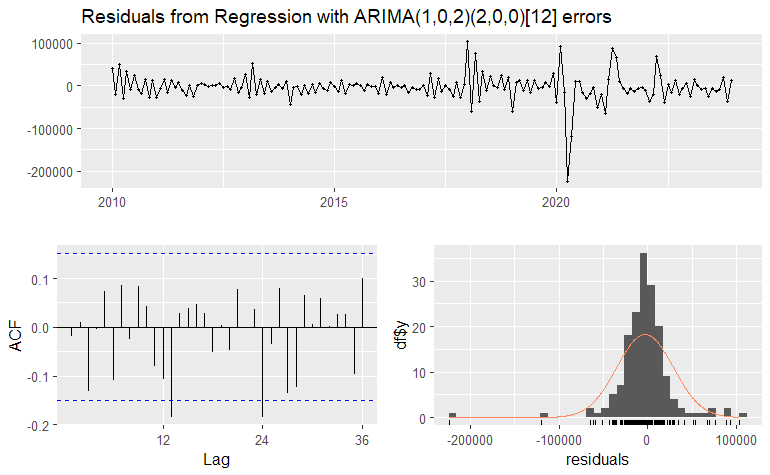
The seasonal model passes. Residuals are stable and small outside 2020, autocorrelations sit inside the confidence bands at nearly every lag, the distribution is approximately normal, and Ljung–Box returns p = 0.0688 — above 0.05, so white noise cannot be rejected. The margin is not generous, but the test is passed.
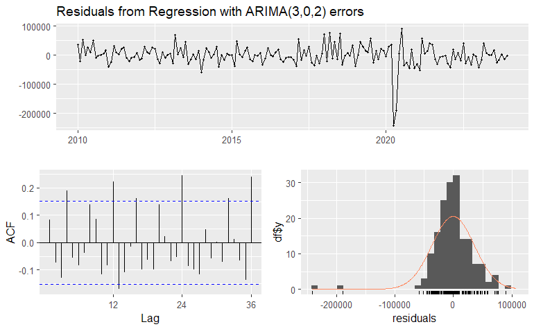
The control model does not. Its residuals fluctuate periodically, several lags breach the confidence bands, and Ljung–Box returns a p-value near zero — white noise is rejected. The leftover structure is the seasonality the specification has no way to represent. This is the point at which the comparison is effectively settled: what follows measures how much that misspecification costs.
07 Forecast results
Both models were used to forecast January–October 2024, ten months held out of estimation entirely.
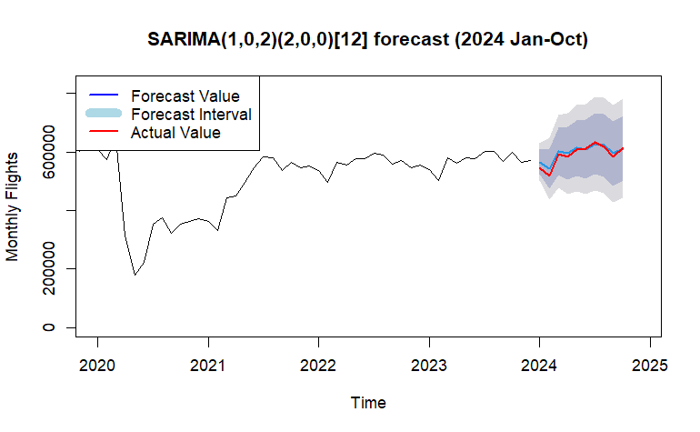
The seasonal forecast tracks the actual series closely and reproduces the shape of the year — the summer peak and the winter trough arrive on schedule and at roughly the right amplitude, not merely the right average level.
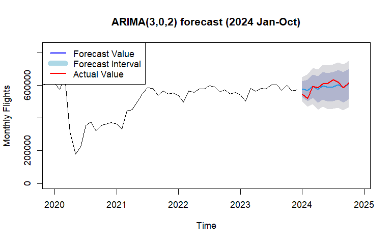
The control model gets the direction right and the shape wrong. It captures the general upward drift but flattens the seasonal swing, so the divergence from actuals is largest exactly where a capacity planner would care most — at the peaks and troughs.
| Model | AIC | BIC | MAPE | MAE | RMSE |
|---|---|---|---|---|---|
| SARIMAX | 3,992.41 | 4,023.65 | 1.72% | 9,776.50 | 11,949.44 |
| ARIMAX | 4,027.05 | 4,058.29 | 3.47% | 20,096.85 | 25,436.12 |
The seasonal model wins on every measure. It fits better in-sample on both information criteria, and its out-of-sample error is roughly half — an average miss of about 9,800 flights a month against 20,100.
08 Limits and next steps
Two constraints bound how far this result travels.
It is a national aggregate. Summing across all reporting carriers averages away the local disturbances — weather, single-airport events, individual carrier decisions — that make station-level series harder to model. At a single airport the series may well not be stationary; a study of Los Angeles International found exactly that and had to difference before fitting (Schneider & Chen, 2020). The accuracy reported here should not be assumed to survive disaggregation to a route or a station.
Two exogenous variables is a thin bridge to the real economy. Income and fuel are the obvious channels, but not the only ones. Tourism indicators, load factors, and policy variables — border measures, subsidy regimes — are plausible additions, and would matter most in precisely the conditions where this specification is weakest: sudden shocks and structural breaks.
The wider point is methodological rather than aviation-specific. Where a series carries a strong and stable seasonal signature, a model that omits it does not simply lose precision — it leaves recoverable structure in the residuals and misattributes that structure to whatever regressors remain. The swapped significance of fuel price between Tables 1 and 2 is that failure made visible.
Data and estimation code available on request. Questions and corrections to jibing@soboaviation.com.
References
- Abdelghany, A., & Guzhva, V. S. (2010). A time-series modelling approach for airport short-term demand forecasting. Journal of Airport Management, 5(1), 72. doi.org/10.69554/BTGX6771
- Abrahams, M. (1983). A service quality model of air travel demand: An empirical study. Transportation Research Part A, 17(5), 385–393. doi.org/10.1016/0191-2607(83)90007-9
- Andreoni, A., & Postorino, M. N. (2006). A multivariate ARIMA model to forecast air transport demand. Association for European Transport.
- Bureau of Transportation Statistics. (2020). Preliminary air traffic data, April 2020: 96% reduction in U.S. airline passengers from 2019. bts.gov
- Bureau of Transportation Statistics. (2024). Arriving flights, Airline Performance — Arrivals database, 01/2010–12/2024 [Dataset]. Sage Data.
- Centers for Disease Control and Prevention. (2024). CDC Museum COVID-19 timeline. cdc.gov
- Gu, W., Guo, B., Zhang, Z., & Lu, H. (2024). Civil aviation passenger traffic forecasting. Sustainability, 16(10), 4110. doi.org/10.3390/su16104110
- Michelmann, J., Schmalz, U., Becker, A., Stroh, F., Behnke, S., & Hornung, M. (2023). Influence of COVID-19 on air travel. Journal of Air Transport Management, 106, 102325. doi.org/10.1016/j.jairtraman.2022.102325
- Schneider, R., & Chen, X. (2020). Predicting flight demand under uncertainty. KSCE Journal of Civil Engineering, 24(2), 635–646. doi.org/10.1007/s12205-020-0857-9
- Tsui, W. H. K., Ozer Balli, H., Gilbey, A., & Gow, H. (2014). Forecasting of Hong Kong airport's passenger throughput. Tourism Management, 42, 62–76. doi.org/10.1016/j.tourman.2013.10.008
- Wadud, Z. (2014). The asymmetric effects of income and fuel price on air transport demand. Transportation Research Part A, 65, 92–102. doi.org/10.1016/j.tra.2014.04.001